Linear Regression is one of the most used statistical models in the industry. The main advantage of linear regression lies in its simplicity and interpretability. Linear regression is used to forecast revenue of a company based on parameters, forecasting player’s growth in sports, predicting the price of a product given the cost of raw materials, predicting crop yield given rainfall and much much more.
During our internship at Ambee, we were given a warm-up task to predict car prices given the dataset. This task strengthened our understanding of feature selection for multivariate linear regression and statistical measures for choosing the right model. You might be wondering why does an environment company makes interns work on a car pricing dataset. At Ambee, we celebrate outside data as much as inside data. That’s what makes us relate things like how a change in pollutants impacts health businesses’ economies of scale, which aren’t seen directly by many but affect indirectly. It is important for a data scientist to gain domain knowledge but it is also important to keep an open mind on external factors that can be directly or indirectly related.
Regression is a statistical technique used to model continuous target variables. It has also been adopted to Machine Learning to predict continuous variables.
Regression models the target variable as a function of independent variables also called as predictors.
Linear Regression fits a straight line to our data. Simple Linear Regression (SLR) models target variable as a function of a single predictor whereas Multivariate Linear Regression (MLR) models target variable as a function of multiple predictors.
Problem Statement
A new car manufacturer is looking to set up business in the US Market. They need to know the factors on which the pricing of a car depends on to take on their competition in the market. The company wants to know the variables the price depends on and to what extent does the variables explain the price of a car.
Business Goal
We need to build a model for the price of a car as a function of explanatory variables. The company will then use it to configure the price of a car according to its features or configure the features according to its price.
In this blog post, we shall go through the process of cleaning the data, understanding our variables and modelling using linear regression.
Let us import our libraries. Numpy is a fast matrix computation library that most of the other libraries depend on and we might need it at some point. Pandas is our data manipulation library and one of the most important libraries in our pipeline. matplotlib and Seaborn are used for plotting graphs.
import numpy as np
import pandas as pd
import matplotlib.pyplot as plt
import seaborn as sns
Let us read our dataset.
cardata=pd.read_csv(r'CarPrice_Assignment.csv')
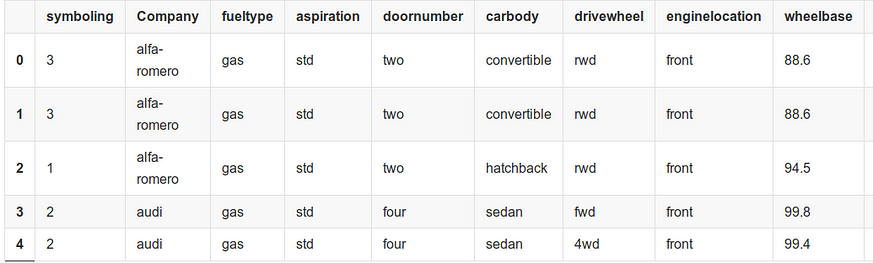
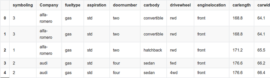
cardata.head()
5 rows × 26 columns
We can use head() to view first five records. We observe that there are a lot of variables and many of them are categorical. So, feature selection will play an important role going forward.
Let us check if there are any missing values.
Turns out there aren’t any. So we do not need to worry about filling any missing values.
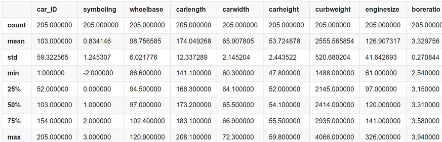
We can get descriptive statistical values using describe() of pandas.
cardata.describe()
Now, we shall do some processing of our data.
1) We only want the company name. So lets split the CarName and extract only company name. We will rename it to Company to avoid confusion.
2) We will calculate total miles per gallon and remove citympg and highwaympg
3) We do not require ID as well so lets remove that as well.
4) We will change the datatype of symboling to string since its a categorical variable and should not be confused to be continuous.
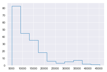
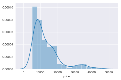
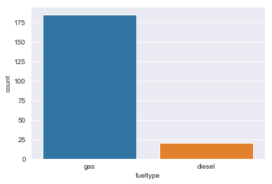
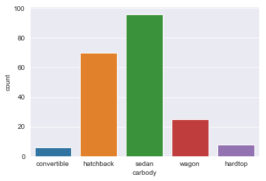
Now, let us explore our data. We will look at how our data is distributed by plotting a histogram. We’ve plotted using both matplotlib and seaborn but both are the same while interpreting.
<matplotlib.axes._subplots.AxesSubplot at 0x7fcd1d20aeb8>
We can see that our data is skewed by looking at the above plots. What this means is that there are more cheaper cars in our dataset than expensive cars.
Mean: 13276.710570731706
Median: 10295.0
Standard Deviation: 7988.85233174315
Variance: 63821761.57839796
Since Mean and Median is not similar, data is skewed as seen in above histogram. There is also high amount of variance in the data.
cardata.price.describe()
count      205.000000
mean     13276.710571
std       7988.852332
min       5118.000000
25%       7788.000000
50%      10295.000000
75%      16503.000000
max      45400.000000
Name: price, dtype: float64
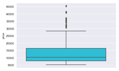
We shall plot a boxplot to see how our price is distributed. Boxplot shows minimum, first quartile(25%), median, third quartile(75%), maximum and outliers (represented using dots).
sns.boxplot(y=cardata.price,color='#13d2f2')
<matplotlib.axes._subplots.AxesSubplot at 0x7fcd1f5b7828>
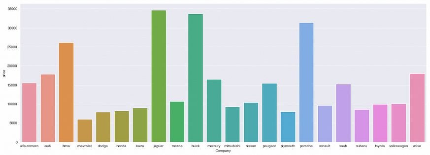
We can see below that most cars in our dataset is manufactured by Toyota.
<matplotlib.axes._subplots.AxesSubplot at 0x7fcd1cb276d8>
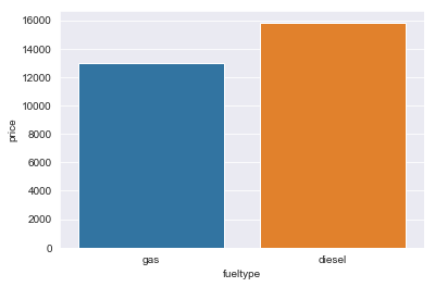
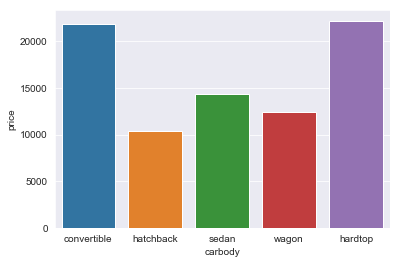
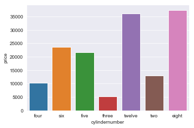
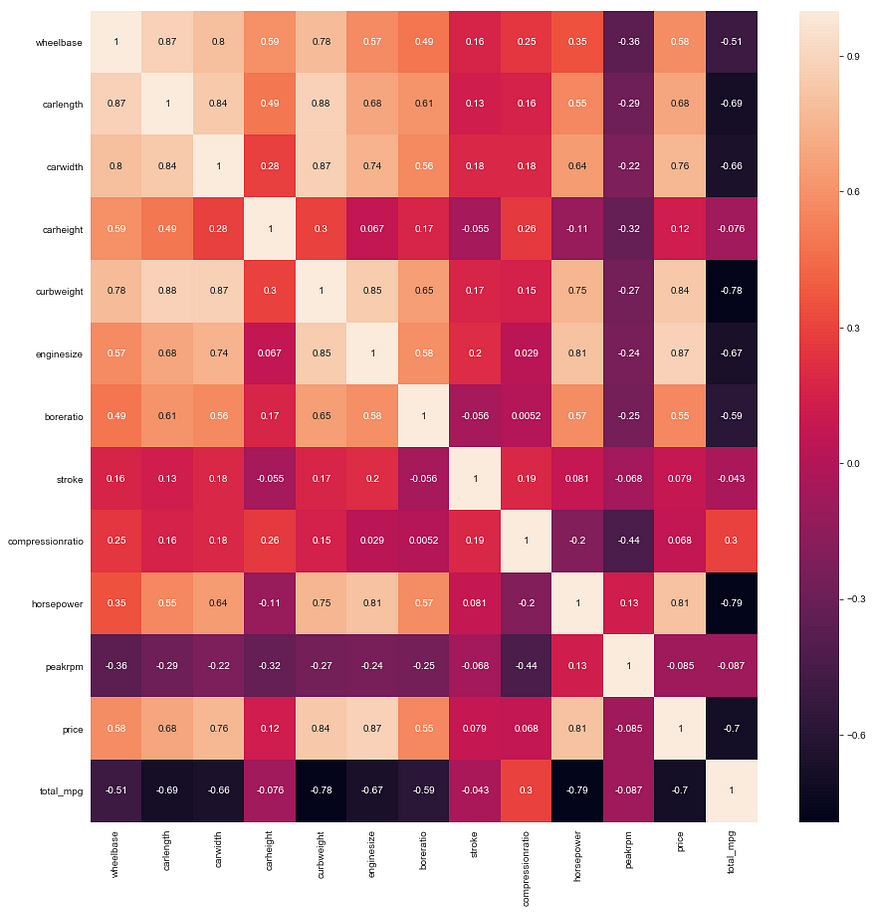
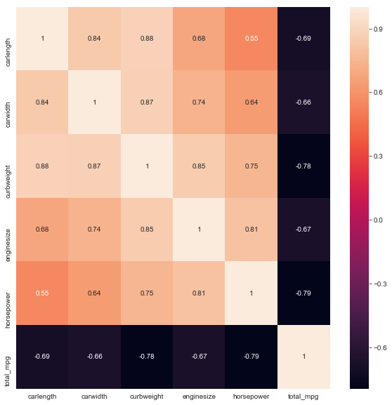
Now, we need to select features using which we can model our price using linear regression. So, we will look at how much correlation each feature has with price. Correlation explains how much two things are related to each other. For example, the amount of rainfall is correlated with how wet your garden is. But, correlation doesn’t always mean causation. Just because your garden is wet doesn’t mean it was due to rain. It can also be the sprinkler or any other source of water. In general, correlation helps us the choose the most important variables to model after.
Now, we shall look for multicollinearity. Two variables are collinear if they are highly correlated. Multicollinearlity happens when there is high correlation between predictors. This is a problem because linear regression doesn’t handle multicollinearity well.
<matplotlib.axes._subplots.AxesSubplot at 0x7fcd1c9be2e8>
We see that enginesize, horsepower,curbweight and totalmpg are highly correlated. We need to choose one predictor among these.
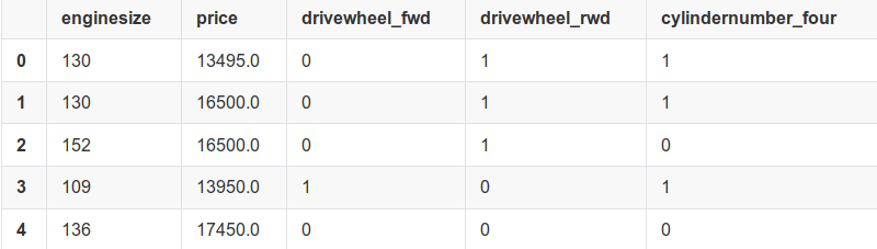
We need to now handle categorical variables. We can convert them to binary variables using get_dummies(). Each value in column becomes a separate column after getting the binarization.
cardata=pd.get_dummies(cardata)
We need to select one predictor from enginesize, horsepower,curbweight and totalmpg. We shall make a simple linear regression model for each predictor.
Before moving ahead, we need to look at some statistical measures to choose best value.
1) p-value helps you determine the significance of your results. The relation is statistically significant if p value is less than 0.05. 2) R2 measures goodness of the fit. Higher R2 score means our model fits the data better. But, with increasing number of features, R2 also increases. So, we need to be careful.
Warnings: [1] Standard Errors assume that the covariance matrix of the errors is correctly specified. [2] The condition number is large, 1.31e+04. This might indicate that there are strong multicollinearity or other numerical problems.
predictors=cardata['total_mpg'] import statsmodels.api as sm predictors= sm.add_constant(predictors) lm_1 = sm.OLS(target,predictors).fit() print(lm_1.summary())
Warnings:
[1] Standard Errors assume that the covariance matrix of the errors is correctly specified.
From the above observations, we can select one of the predictors. Since enginesize has highest R2 value and P value of 0, we can select that. The reason for selecting just one of the above predictors is due to high amount of multicollinearity between them. We shall drop the rest.
<matplotlib.axes._subplots.AxesSubplot at 0x7fcd1815cbe0>
We will also drop all columns having correlation to price around 0.5. We will also drop carlength and carwidth since they are highly correlated to each other and significantly correlated with enginesize.
Warnings:
[1] Standard Errors assume that the covariance matrix of the errors is correctly specified.
We get a decent model with R2 score of 0.76 only using enginesize. We will now add more variables to it to see if it improves our model.
Let us see if adding forward wheel drive or backward wheel drive improves our model.
predictors2=predictors[['enginesize','drivewheel_fwd']] import statsmodels.api as sm predictors2= sm.add_constant(predictors2) lm_2 = sm.OLS(target,predictors2).fit() print(lm_2.summary())
Warnings: [1] Standard Errors assume that the covariance matrix of the errors is correctly specified. [2] The condition number is large, 1.13e+03. This might indicate that there are strong multicollinearity or other numerical problems.
We get a warning saying that there is a strong multicollinearity. It can be explained since both forward wheel drive and backward wheel drives do not coexist. We see that our p values increase beyond 0.005. So, we cannot go with above predictors
We will add cylindernumber_four variable to our existing models and see if it improves our model.
predictors5=predictors[['enginesize','drivewheel_rwd','cylindernumber_four']] import statsmodels.api as sm predictors5= sm.add_constant(predictors5) lm_5 = sm.OLS(target,predictors5).fit() print(lm_5.summary())
Warnings:
[1] Standard Errors assume that the covariance matrix of the errors is correctly specified.
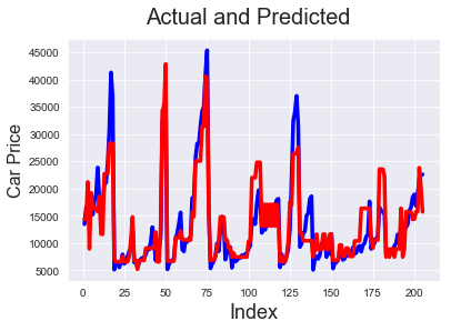
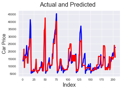
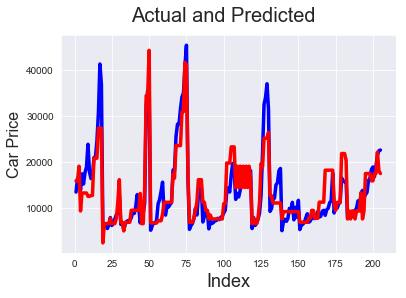
Now, let us plot our predictions to see how our models perform.
pred=lm_6.predict(predictors6)
# Actual vs Predicted
c = [i for i in range(1,206,1)]
fig = plt.figure()
plt.plot(c,target, color="blue", linewidth=3.5, linestyle="-")     #Plotting Actual
plt.plot(c,pred, color="red",  linewidth=3.5, linestyle="-")  #Plotting predicted
fig.suptitle('Actual and Predicted', fontsize=20)              # Plot heading
plt.xlabel('Index', fontsize=18)                               # X-label
plt.ylabel('Car Price', fontsize=16)
Text(0, 0.5, 'Car Price')
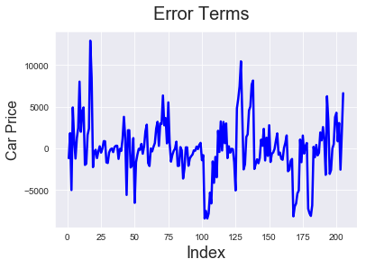
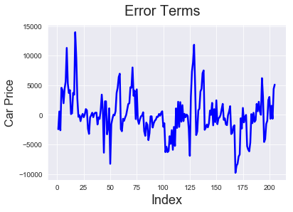
# Error terms
c = [i for i in range(1,206,1)]
fig = plt.figure()
plt.plot(c,target-pred, color="blue", linewidth=2.5, linestyle="-")
fig.suptitle('Error Terms', fontsize=20)              # Plot heading
plt.xlabel('Index', fontsize=18)                      # X-label
plt.ylabel('Car Price', fontsize=16)
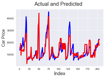
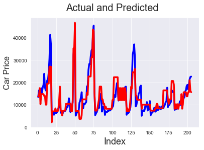
# Actual vs Predicted
c = [i for i in range(1,206,1)]
fig = plt.figure()
plt.plot(c,target, color="blue", linewidth=3.5, linestyle="-")     #Plotting Actual
plt.plot(c,pred, color="red",  linewidth=3.5, linestyle="-")  #Plotting predicted
fig.suptitle('Actual and Predicted', fontsize=20)              # Plot heading
plt.xlabel('Index', fontsize=18)                               # X-label
plt.ylabel('Car Price', fontsize=16)
Text(0, 0.5, 'Car Price')
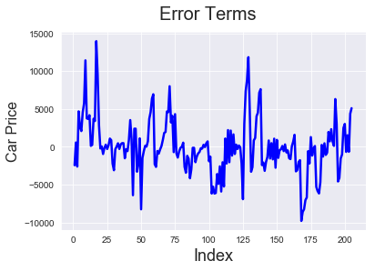
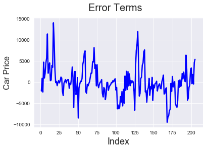
# Error terms
c = [i for i in range(1,206,1)]
fig = plt.figure()
plt.plot(c,target-pred, color="blue", linewidth=2.5, linestyle="-")
fig.suptitle('Error Terms', fontsize=20)              # Plot heading
plt.xlabel('Index', fontsize=18)                      # X-label
plt.ylabel('Car Price', fontsize=16)
# Actual vs Predicted
c = [i for i in range(1,206,1)]
fig = plt.figure()
plt.plot(c,target, color="blue", linewidth=3.5, linestyle="-")     #Plotting Actual
plt.plot(c,pred, color="red",  linewidth=3.5, linestyle="-")  #Plotting predicted
fig.suptitle('Actual and Predicted', fontsize=20)              # Plot heading
plt.xlabel('Index', fontsize=18)                               # X-label
plt.ylabel('Car Price', fontsize=16)
Text(0, 0.5, 'Car Price')
# Error terms
c = [i for i in range(1,206,1)]
fig = plt.figure()
plt.plot(c,target-pred, color="blue", linewidth=2.5, linestyle="-")
fig.suptitle('Error Terms', fontsize=20)              # Plot heading
plt.xlabel('Index', fontsize=18)                      # X-label
plt.ylabel('Car Price', fontsize=16)
We can see that models 6 and 5 predict the price pretty well. So the solution for our problem statement is to look at enginesize, forward/backward wheel drive and see if the number of cylinders is 4 (which has negative correlation with price) to determine the price,
This task was done by Pareekshith US Katti and N Nithin Srivatsav while doing internship at Ambee.
Most teams across IT organizations need access to virtual machines (VM), or Elastic Compute Cloud (EC2), for various developmental activities in the AWS ecosystem. Providing Secure Shell (SSH) access with well-defined security policies and roles Read more…
We at Ambee are always dealing with large chunks of data ( ~4TB / day ). Now that’s huge. You obviously can’t handle it using pandas ( or can you? ) Here is where the Read more…
Idea in Brief: Electric Vehicles (EVs) have become the next big solution for increasing efficiency in road transport and decreasing air pollution rates. Even though EVs are still at a nascent stage, they have begun Read more…