Okay.. it’s been a long time now that we have got back together.

In the Part-1 of our EDA we did some pre-pepping with the data.

No intro, no nothing. Let’s dive right in!!

Here is our problem statement again.

The task is to analyze ball by ball data from all the way from 2008 to 2019.

Using this we need to come up with analysis to form your own dream team for IPL. For year 2016, 2017 and 2018, we need to find out :

1. Find out most valuable player – explain why
2. Find out most consistent batsman – explain why
3. Find out most consistent bowler – explain why
4. Find out, worst player – explain why
5. Find out worst batsmen – explain why
6. Find out worst bowler – explain why
7. Rank top 25 players for the year 2016 to 2019
8. Identify most improved player from 2018 to 2019
9. Find out which stadium had the most runs and which scored the least
10. Which bowler gave the least runs and took most wickets.(Economy)
11. Design a super awesome dream team for 2020.

Data Analysis

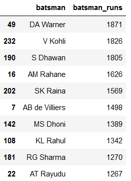
A lil bit of mushing here and there…

df=Deliveries.loc[Deliveries['season']>=2016]
df=df.groupby('batsman').sum()
df.reset_index(level=0, inplace=True)
df=df[['batsman','batsman_runs']]
df.sort_values(by=['batsman_runs'],ascending=False,inplace=True)
df.head(10)

Let’s just take a quick overview of who has the highest runs and wickets.​​

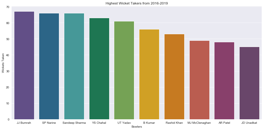
df1=Deliveries.loc[Deliveries['season']>=2016]
df1=df1.groupby('bowler').sum()
df1.reset_index(level=0, inplace=True)
df1=df1[['bowler','type_out']]
df1.sort_values(by=['type_out'],ascending=False,inplace=True)
df1.head(10) 

Now the Graphical representation.

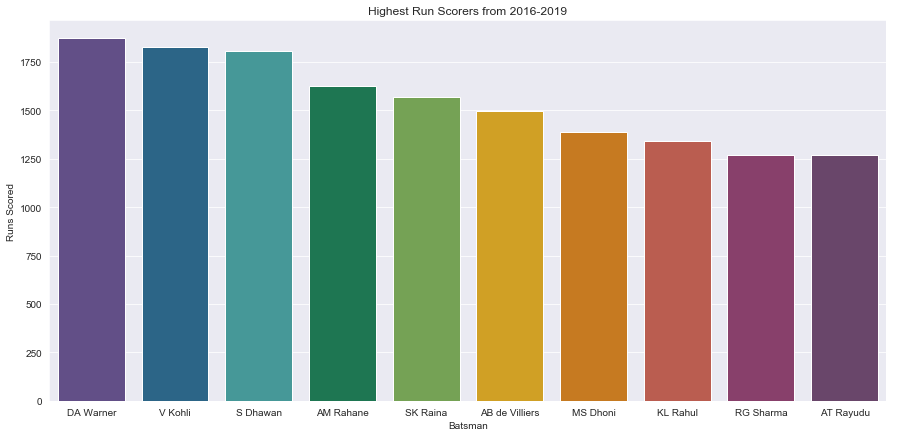
import palettable
sns.set_style('darkgrid')
pal=palettable.cartocolors.qualitative.Prism_10.mpl_colors
plt.figure(figsize=[15,7])
plt.title('Highest Run Scorers from 2016-2019')
ax=sns.barplot(x='batsman',y='batsman_runs',data=df.head(10),palette=pal)
t=ax.set(xlabel='Batsman',ylabel='Runs Scored')

pal=palettable.cartocolors.qualitative.Prism_10.mpl_colors
plt.figure(figsize=[15,7])
plt.title('Highest Wicket Takers from 2016-2019')
sns.set_style('darkgrid')
ax=sns.barplot(x='bowler',y='type_out',data=df1.head(10),palette=pal)
t=ax.set(xlabel='Bowlers',ylabel='Wickets Taken')

Calculating MVP Values for Players

There are a few criteria of how MVPs of players are calculated according to IPL and BCCI. Since it is quite a complex algorithm, let’s define our own algorithm in the lines of it.

def mvpbat(x):
    if x==4: #If  it is a four assign 2.5
        return 2.5
    elif x==6: #If it is a six assign 3.5
        return 3.5
    else:
        return 0
def mvpbowl(x): #If he takes a wicket assign 2.5
    if x==1:
        return 2.5
    else:
        return 0
def mvpdotball(x): #Assign 1 for every dot ball.
    if x==0:
        return 1
    else:
        return 0
def mvpfield(x): #If he has taken a catch or any other type of wicket.
    if x=='0':
        return 0
    else:
        return 2.5
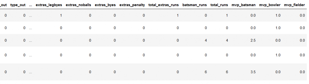
Deliveries['mvp_batsman'] = [mvpbat(x) for x in Deliveries['batsman_runs']]
Deliveries['mvp_bowler'] = [mvpbowl(x) for x in Deliveries['type_out']]
Deliveries['mvp_dot'] = [mvpdotball(x) for x in Deliveries['batsman_runs']]
Deliveries['mvp_fielder']= [mvpfield(x) for x in Deliveries['fielder_caught_out']]
Deliveries['mvp_bowler']+=Deliveries['mvp_dot']
Deliveries.drop('mvp_dot',axis=1,inplace=True)

Deliveries.head()

Creating Dataframes for MVPs in Batting, Bowling and Overall

mvpbat=Deliveries.loc[Deliveries['season']>=2016]
mvpbat=mvpbat.groupby(['batsman','season']).sum()
mvpbat.reset_index(level=(0,1), inplace=True)
​
mvpbat.sort_values(by=['batsman_runs'],ascending=False,inplace=True)
mvpbat.head(10)
mvpbat.drop(['mvp_bowler','bowled_over','type_out','extras_wides',
'extras_legbyes','extras_noballs','extras_byes','total_extras_runs',
'total_runs','extras_penalty'],axis=1,inplace=True)
mvpbat.rename(index=str,columns={'batsman':'player'},inplace=True)
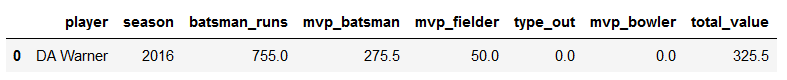
mvpbat.head()

mvpbowl=Deliveries.loc[Deliveries['season']>=2016]
mvpbowl=mvpbowl.groupby(['bowler','season']).sum()
mvpbowl.reset_index(level=(0,1), inplace=True)
​
mvpbowl.sort_values(by=['type_out'],ascending=False,inplace=True)
mvpbowl.head(10)
mvpbowl.drop(['mvp_batsman','mvp_fielder','bowled_over','batsman_runs','extras_wides',
'extras_legbyes','extras_noballs','extras_byes','total_extras_runs',
'total_runs','extras_penalty'],axis=1,inplace=True)
mvpbowl.rename(index=str,columns={'bowler':'player'},inplace=True)
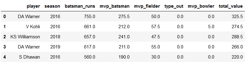
mvp=mvpbat.merge(mvpbowl,how='outer')
mvp.fillna(0,inplace=True)
mvp['total_value']=mvp['mvp_batsman']+mvp['mvp_bowler']+mvp['mvp_fielder'] 
mvp.head() 

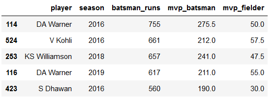
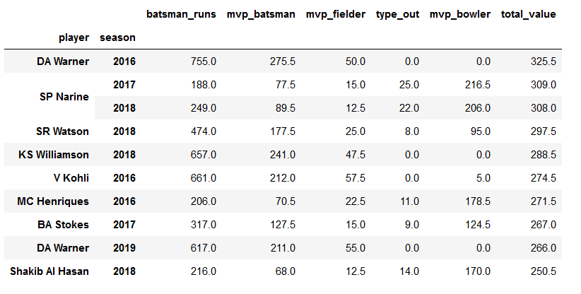
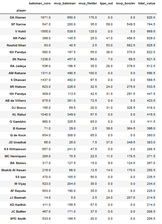
mvp.groupby(['player','season']).sum().sort_values('total_value',ascending=False).head(10)

If we take a closer look at the above table, it is quite unbiased because there are batsman, bowlers and all rounders, hence our method of assign MVP isn’t a flaw. Once we have calculated the total values, lets start completing our objective. Let’s first group everything into seasons.

Dividing MVP table wrt seasons

season2016=mvp[mvp['season']==2016]
season2017=mvp[mvp['season']==2017]
season2018=mvp[mvp['season']==2018]
season2019=mvp[mvp['season']==2019]
​
season2016bat=mvpbat[mvpbat['season']==2016]
season2017bat=mvpbat[mvpbat['season']==2017]
season2018bat=mvpbat[mvpbat['season']==2018]
season2019bat=mvpbat[mvpbat['season']==2019]
​
season2016bowl=mvpbowl[mvpbowl['season']==2016]
season2017bowl=mvpbowl[mvpbowl['season']==2017]
season2018bowl=mvpbowl[mvpbowl['season']==2018]
season2019bowl=mvpbowl[mvpbowl['season']==2019]

Finding MVP for each season

#Most Valuable Player for each season
season2016[season2016['total_value']==max(season2016['total_value'])]

season2017[season2017['total_value']==max(season2017['total_value'])]

season2018[season2018['total_value']==max(season2018['total_value'])]

Objective 1 done.

Finding Most Consistent Batsman and Bowler

#Most Consistent Batsman
top10bat=pd.concat([season2016bat.sort_values('mvp_batsman',ascending=False).head(10),
season2017bat.sort_values('mvp_batsman',ascending=False).head(10),
season2018bat.sort_values('mvp_batsman',ascending=False).head(10)])

top10bat.groupby('player').sum().sort_values('mvp_batsman',ascending=False)['mvp_batsman'].head(1)

Output:
player
AM Rahane    490.5
Name: mvp_batsman, dtype: float64

#Most Consistent Bowler
top10bowl=pd.concat([season2016bowl.sort_values('mvp_bowler',ascending=False).head(10),
season2017bowl.sort_values('mvp_bowler',ascending=False).head(10),
season2018bowl.sort_values('mvp_bowler',ascending=False).head(10)])

top10bowl.groupby('player').sum().sort_values('mvp_bowler',ascending=False)['mvp_bowler'].head(1)

Output: 
player
JJ Bumrah    541.5
Name: mvp_bowler, dtype: float64

Objective 2 and 3 done.

Worst Player, Batsman and Bowler

#Worst Player
season2016[season2016['total_value']==min(season2016['total_value'])].tail(1)

season2017[season2017['total_value']==min(season2017['total_value'])].tail(1)

season2018[season2018['total_value']==min(season2018['total_value'])].tail(1)

#Worst Batsman
season2016bat[(season2016bat['mvp_batsman']==min(season2016bat['mvp_batsman']))].tail(1)

season2017bat[(season2017bat['mvp_batsman']==min(season2017bat['mvp_batsman']))].tail(1)

season2018bat[(season2018bat['mvp_batsman']==min(season2018bat['mvp_batsman']))].tail(1)

#Worst Bowler
season2016bowl[(season2016bowl['mvp_bowler']==min(season2016bowl['mvp_bowler']))].tail(1)

season2017bowl[(season2017bowl['mvp_bowler']==min(season2017bowl['mvp_bowler']))].tail(1)

season2018bowl[(season2018bowl['mvp_bowler']==min(season2018bowl['mvp_bowler']))].tail(1)

Objective 4, 5 and 6 done.

Top 25 Players Each Season

#Top 25 For Each Year
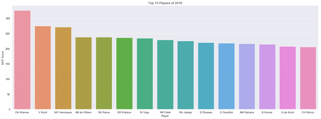
top25=season2016.sort_values('total_value',ascending=False).head(25)

plt.figure(figsize=[20,7])
plt.title('Top 15 Players of 2016')
sns.set_style('darkgrid')
ax=sns.barplot(x='player',y='total_value',data=top25.head(15))
t=ax.set(xlabel='Player',ylabel='MVP Score')

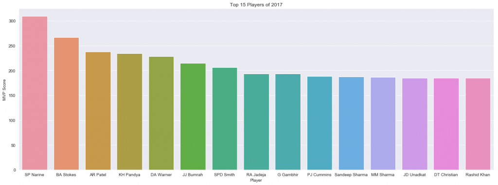
top25=season2017.sort_values('total_value',ascending=False).head(25)

plt.figure(figsize=[20,7])
plt.title('Top 15 Players of 2017')
sns.set_style('darkgrid')
ax=sns.barplot(x='player',y='total_value',data=top25.head(15))
t=ax.set(xlabel='Player',ylabel='MVP Score')

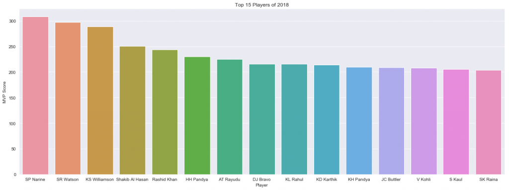
top25=season2018.sort_values('total_value',ascending=False).head(25)

plt.figure(figsize=[20,7])
plt.title('Top 15 Players of 2018')
sns.set_style('darkgrid')
ax=sns.barplot(x='player',y='total_value',data=top25.head(15))
t=ax.set(xlabel='Player',ylabel='MVP Score')

top25=season2019.sort_values('total_value',ascending=False).head(25)

plt.figure(figsize=[20,7])
plt.title('Top 15 Players of 2019')
sns.set_style('darkgrid')
ax=sns.barplot(x='player',y='total_value',data=top25.head(15))
t=ax.set(xlabel='Player',ylabel='MVP Score')

Objective 7 done.

Most Improved Player from 2018 to 2019

mvpimproved=season2018.merge(season2019,left_on='player',right_on='player')

mvpimproved=mvpimproved[['player','total_value_x','total_value_y']]
mvpimproved['improvement']=mvpimproved['total_value_y']-mvpimproved['total_value_x']
player=mvpimproved.sort_values('improvement',ascending=False).head(1)
player 

Objective 8 done. Now we have to work with Matches.csv.

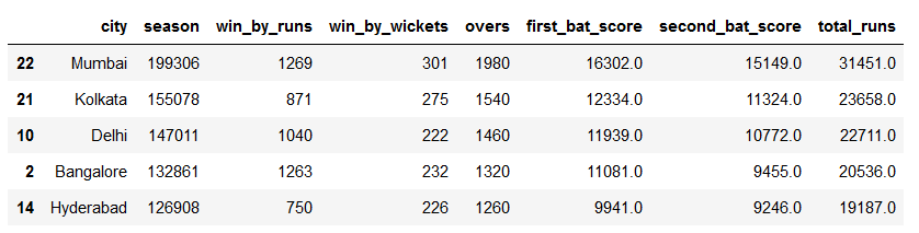
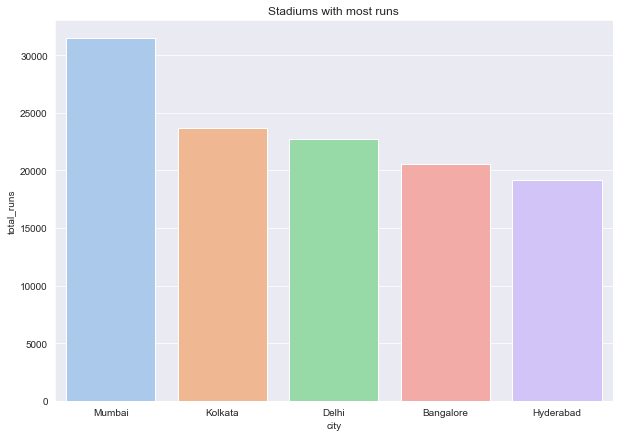
Stadium=Matches.groupby('city').sum()
Stadium['total_runs']=Stadium['first_bat_score']+Stadium['second_bat_score']
Stadium.reset_index(inplace=True)

Stadium=Stadium.sort_values('total_runs',ascending=False).head()
Stadium

A simple bar plot.

plt.figure(figsize=[10,7])
plt.title('Stadiums with most runs')
ax=sns.barplot('city','total_runs',data=Stadium.head(),palette='pastel')

Objective 9 done! For the 10th objective we need to calculate the economy of the bowlers.

Deliveries['bowled_over']=[1 for x in Deliveries['bowled_over']]
#Converting into 1 if they have taken a wicket.

bowler=Deliveries.groupby('bowler').sum()
bowler=bowler[['bowled_over','type_out','total_runs']]

bowler['economy']=6*bowler['total_runs']/bowler['bowled_over']
bowler['average']=bowler['total_runs']/bowler['type_out']
#Calculating economy and average.

bowler=bowler[bowler['bowled_over']>300]
bowler['eco_norm']=(bowler['economy']-bowler['economy'].mean())/bowler['economy'].std()
bowler['avg_norm']=(bowler['average']-bowler['average'].mean())/bowler['average'].std()
bowler['wicket_to_runs']=bowler['eco_norm']+bowler['avg_norm']
bowler=bowler.sort_values('wicket_to_runs')
bowler.reset_index(inplace=True)

from palettable.colorbrewer.qualitative import Paired_12_r
plt.figure(figsize=[20,7])
plt.title('Bowlers who give least runs and take up more wicket')
sns.set_style('darkgrid')
ax=sns.barplot(x='bowler',y='wicket_to_runs',data=bowler.head(10),palette=Paired_12_r.mpl_colors)
t=ax.set(xlabel='Bowler',ylabel='Balance b/w Average and Economy (Lower the better)')

Objective 10 done.

Dream Team for IPL 2020

Now this is the most exciting part. Solving problems like these in data science not only requires coding skills and overview of the data, it also requires that we have an excellent knowledge about the domain we are working on.

Criteria for choosing players

• Maximum of 4 foreign players
• 4 Bowlers
• 4 Batsman
• 2 Allrounders (one bowling allrounder and one batting allrounder)
• 1 Wicket Keeper Batsman

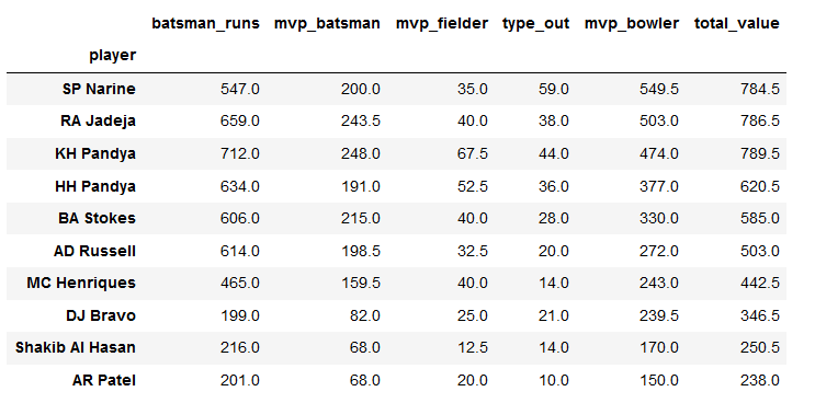
# Start By Looking at Most Consistent Players For Seasons from 2016-2019
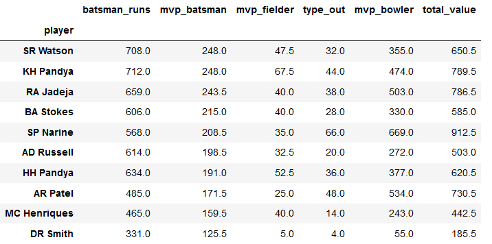
consistent_players=pd.concat([season2016.sort_values('total_value',ascending=False).head(20),
                 season2017.sort_values('total_value',ascending=False).head(20),
                 season2018.sort_values('total_value',ascending=False).head(20),
                 season2019.sort_values('total_value',ascending=False).head(20)])
consistent_players_total=consistent_players.groupby('player').sum().sort_values('total_value',ascending=False)
consistent_players_total.drop('season',axis=1,inplace=True)

consistent_players_total.head(30)

consistent_players_total.sort_values('mvp_batsman',ascending=False).head(30)

consistent_players_total.sort_values('mvp_bowler',ascending=False).head(30)

From the above data, we need to choose

• 4 Pure Batsmen
• 4 Bowlers
• 2 Allrounders
• 1 Wicket Keeper
• Maximum of 4 Overseas Players

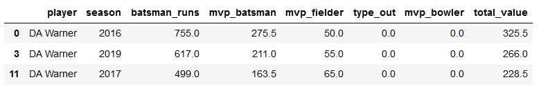
DAWarner=mvp[mvp['player']=='DA Warner']
DAWarner

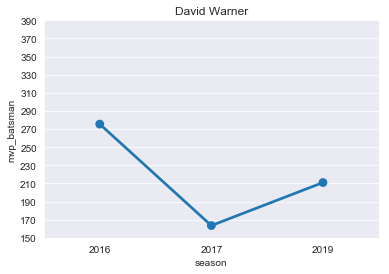
plt.title("David Warner")
ax=sns.pointplot(x='season',y='mvp_batsman',data=DAWarner)
ticks=np.arange(150,400,step=20)
ax=ax.set(yticks=ticks)

We select David Warner as our first foreign player and We need to select 10 more players and 3 more overseas players. Team So Far:

1. David Warner

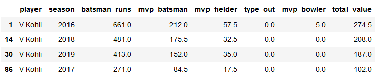
VK=mvp[mvp['player']=='V Kohli']
VK

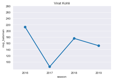
plt.title("Virat Kohli")
ax=sns.pointplot(x='season',y='mvp_batsman',data=VK)
ticks=np.arange(100,300,step=20)
ax=ax.set(yticks=ticks)

Team So Far:

1. David Warner
2. Virat Kohli

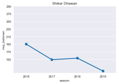
SD=mvp[mvp['player']=='S Dhawan']
SD

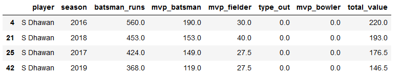
plt.title("Shikar Dhawan")
ax=sns.pointplot(x='season',y='mvp_batsman',data=SD)
ticks=np.arange(150,300,step=20)
ax=ax.set(yticks=ticks)

Team So Far:

1. D Warner
2. S Dhawan
3. V Kohli

We have picked our top order. We will now pick out Middle Order For that we require: 2 Batsman and 1 Wicket Keeper Batsman. We have 3 overseas players. We will Skip AM Rahane since he is a top order batsman and we’ve got it covered. Let us have him as backup. We shall have our next MVP Batsman KL Rahul as backup as well.

SR=consistent_players[consistent_players['player']=='SK Raina']
SR

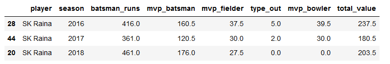
plt.title("Suresh Raina")
ax=sns.pointplot(x='season',y='mvp_batsman',data=SR)
ticks=np.arange(100,300,step=20)
ax=ax.set(yticks=ticks)

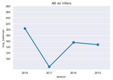
ABD=mvp[mvp['player']=='AB de Villiers']
ABD

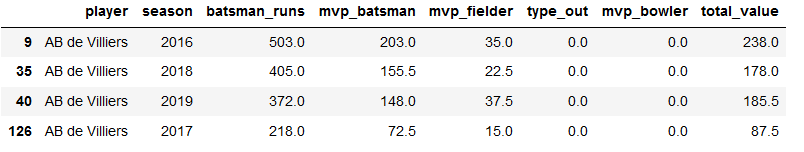
plt.title("AB de Villers")
ax=sns.pointplot(x='season',y='mvp_batsman',data=ABD)
ticks=np.arange(100,300,step=20)
ax=ax.set(yticks=ticks)

We have picked 5 batsmen so far, two of which are overseas players Batting Lineup:

1. D Warner
2. S Dhawan
3. V Kohli
4. Ab de Villers
5. Suresh Raina

Now, we need to pick a wicket keeper. We have Q deKock who is the highest ranked wicket keeper in our most consistent batsmen dataframe. But choosing him would mean we are left with 1 overseas player. So, we will choose the next best wicket keeper who is an Indian, RR Pant

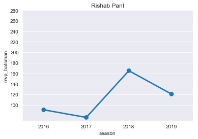
RP=mvp[mvp['player']=='RR Pant']
RP

plt.title("Rishab Pant")
ax=sns.pointplot(x='season',y='mvp_batsman',data=RP)
ticks=np.arange(100,300,step=20)
ax=ax.set(yticks=ticks)

Batting Lineup so far:

1. D Warner
2. S Dhawan
3. V Kohli
4. Ab de Villers
5. Suresh Raina
6. Rishab Pant

We have 2 overseas players remaining. We need to pick 1 batting allrounder, 1 bowling allrounder, 3 pure bowlers. To choose the batting allrounder, we will look at the players who have highest mvp_bowler value among top 30 batsmen for seasons from 2016-2019

top25bat=pd.concat([season2016.sort_values('mvp_batsman',ascending=False).head(50),
                 season2017.sort_values('mvp_batsman',ascending=False).head(50),
                 season2018.sort_values('mvp_batsman',ascending=False).head(50),
                 season2019.sort_values('mvp_batsman',ascending=False).head(50)])
top25bat.drop('season',axis=1,inplace=True)
top25bat.groupby('player').sum().sort_values('mvp_bowler',ascending=False).head(10)

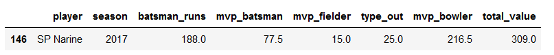
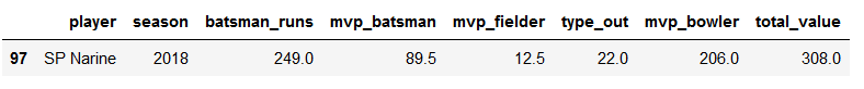
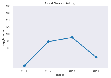
SP=mvp[mvp['player']=='SP Narine']
SP

plt.title("Sunil Narine Batting")
ax=sns.pointplot(x='season',y='mvp_batsman',data=SP)
ticks=np.arange(60,200,step=20)
ax=ax.set(yticks=ticks)

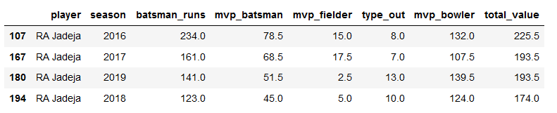
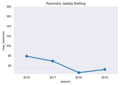
RJ=mvp[mvp['player']=='RA Jadeja']
RJ

plt.title("Ravindra Jadeja Batting")
ax=sns.pointplot(x='season',y='mvp_batsman',data=RJ)
ticks=np.arange(60,200,step=20)
ax=ax.set(yticks=ticks)

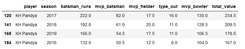
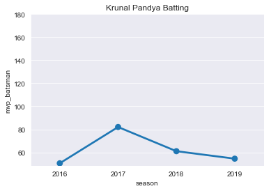
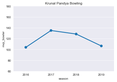
KP=mvp[mvp['player']=='KH Pandya']
KP

plt.title("Krunal Pandya Batting")
ax=sns.pointplot(x='season',y='mvp_batsman',data=KP)
ticks=np.arange(60,200,step=20)
ax=ax.set(yticks=ticks)

HP=mvp[mvp['player']=='HH Pandya']
HP

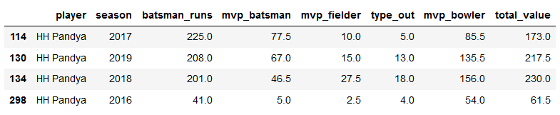
plt.title("Hardik Pandya Batting")
ax=sns.pointplot(x='season',y='mvp_batsman',data=KP)
ticks=np.arange(60,300,step=20)
ax=ax.set(yticks=ticks)

If we observe the graphs of 4 players for mvp_batsman, we observe that HH Pandya and KH Pandya are the most consistent with mvp_bat around 60. RA Jadeja and SR Narine have a dip in form. If we chose HH Pandya, We can need to choose an extra spinner. If we chose KH Pandya, We can need to choose an extra pacer. Team so far:

1. D Warner
2. S Dhawan
3. V Kohli
4. Ab de Villers
5. Suresh Raina
6. Rishab Pant
7. Hardik/Krunal Pandya

We now need to choose a bowling all rounder. To choose the bowling all rounder, we will look at the players who have highest mvp_batsman value among top 30 bowlers for seasons from 2016-2019

top25bowl=pd.concat([season2016.sort_values('mvp_bowler',ascending=False).head(50),
                 season2017.sort_values('mvp_bowler',ascending=False).head(50),
                 season2018.sort_values('mvp_bowler',ascending=False).head(50),
                 season2019.sort_values('mvp_bowler',ascending=False).head(50)])
top25bowl.drop('season',axis=1,inplace=True)
top25bowl.groupby('player').sum().sort_values('mvp_batsman',ascending=False).head(10)

SR Watson is retired. Since we already have KH Pandya shortlisted, we can go with him.

plt.title("Krunal Pandya Bowling")
ax=sns.pointplot(x='season',y='mvp_bowler',data=KP)
ticks=np.arange(60,200,step=20)
ax=ax.set(yticks=ticks)

Team so far:

1. D Warner
2. S Dhawan
3. V Kohli
4. Ab de Villers
5. Suresh Raina
6. Rishab Pant
7. Hardik Pandya
8. Krunal Pandya

We need to choose 3 bowlers and we still have 2 overseas players remaining. We can go with either 2 spinners or 2 pacers. If we look at top 2 in most consistent bowlers list, we have Rashid Khan and SR Narine. Both are overseas players and we can afford to pick both of them are overseas players and we can afford to pick both of them.

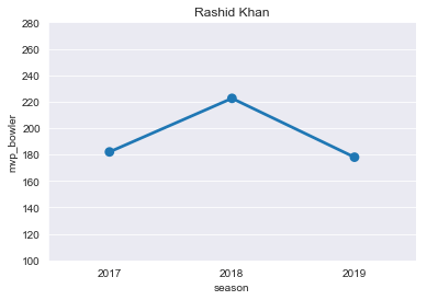
RK=mvp[mvp['player']=='Rashid Khan']
RK

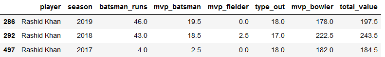
plt.title("Rashid Khan")
ax=sns.pointplot(x='season',y='mvp_bowler',data=RK)
ticks=np.arange(100,300,step=20)
ax=ax.set(yticks=ticks)

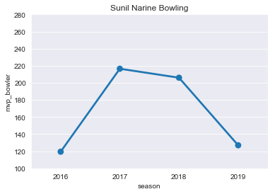
plt.title("Sunil Narine Bowling")
ax=sns.pointplot(x='season',y='mvp_bowler',data=SP)
ticks=np.arange(100,300,step=20)
ax=ax.set(yticks=ticks)

We see a dip in form of Sunil Narine from 2017. We shall go with Rashid Khan as of now and keep Sunil Narine as a backup. We have to pick 2 more bowlers and atleast one pacer and one more overseas player can be accommodated. Highest ranked pace bowler is B Kumar in our list. Batting Lineup:

1. D Warner
2. S Dhawan
3. V Kohli
4. Ab de Villers
5. Suresh Raina
6. Rishab Pant
7. Hardik Pandya
8. Krunal Pandya
9. Rashid Khan

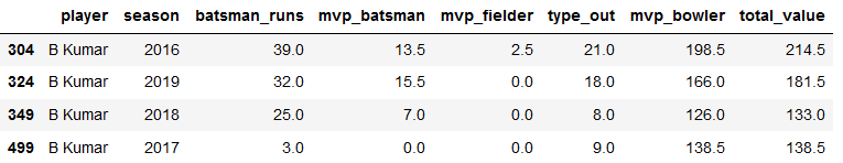
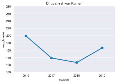
BK=mvp[mvp['player']=='B Kumar']
BK

plt.title("Bhuvaneshwar Kumar")
ax=sns.pointplot(x='season',y='mvp_bowler',data=BK)
ticks=np.arange(100,300,step=20)
ax=ax.set(yticks=ticks)

Batting Lineup:

1. D Warner
2. S Dhawan
3. V Kohli
4. Ab de Villers
5. Suresh Raina
6. Rishab Pant
7. Hardik Pandya
8. Krunal Pandya
9. Rashid Khan
10. Bhuvaneshwar Kumar

We now need to pick another bowler. If we go with Pacer, we can go with JD Unadkat, DJ Bravo or JJ Bumrah. We can also go with Sunil Narine if we want a spinner

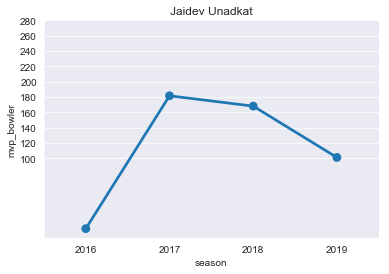
JU=mvp[mvp['player']=='JD Unadkat']
JU

plt.title("Jaidev Unadkat")
ax=sns.pointplot(x='season',y='mvp_bowler',data=JU)
ticks=np.arange(100,300,step=20)
ax=ax.set(yticks=ticks)

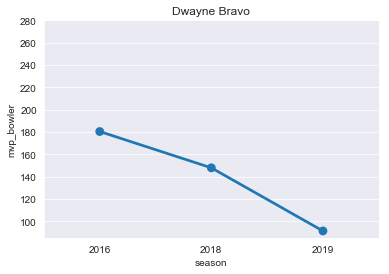
DJ=mvp[mvp['player']=='DJ Bravo']
DJ

plt.title("Dwayne Bravo")
ax=sns.pointplot(x='season',y='mvp_bowler',data=DJ)
ticks=np.arange(100,300,step=20)
ax=ax.set(yticks=ticks)

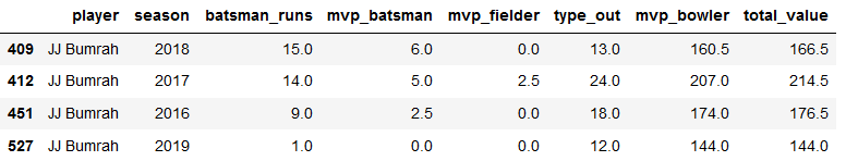
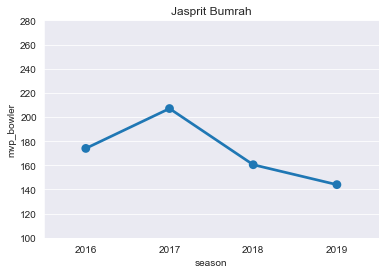
JB=mvp[mvp['player']=='JJ Bumrah']
JB

plt.title("Jasprit Bumrah")
ax=sns.pointplot(x='season',y='mvp_bowler',data=JB)
ticks=np.arange(100,300,step=20)
ax=ax.set(yticks=ticks)

Using the graph above, we can go with JJ Bumrah. So, our playing 11 is, Batting Lineup:

1. D Warner
2. S Dhawan
3. V Kohli
4. Ab de Villers
5. Suresh Raina
6. Rishab Pant
7. Hardik Pandya
8. Krunal Pandya
9. Rashid Khan
10. Bhuvaneshwar Kumar
11. Jasprith Bumrah

Bench:

1. Sunil Narine
2. AM Rahane
3. Quinton de Kock
4. KL Rahul

Objective 11 completed.​

Winding up

​ So as we can observe Exploratory Data Analysis is used to gain insights for some valuable purpose. It requires domain knowledge, overview of data and a lil bit of experience which we shall gain eventually by solving more problems. Data science is a fun domain in computer science and rapidly expanding, and EDA plays a small part. Now that we got this covered, we can move over to other interesting stuff on our pathway to Super awesome Data Scientists. We (Pareekshith and Nithin) were more than happy to have interned under Ambee, especially keeping in mind about the problem they are trying to solve. Until next time. Ba-byee!!